Visualizing Intertextuality
About the Project
This is a project to visualize intertexts and intertextual relationships in Latin poetry. The project is explained in detail below, in terms that should be equally accessible to scholars and students of Latin poetry with no background in coding and Digital Humanities experts—including those with no background in Latin—although some portions of the discussion are directed more towards one group or the other. (Interested parties can also view the code on GitHub.)
Background: What is Intertextuality?
Within the scholarly field of Latin poetry, “intertextuality” is a commonly-addressed concept. The term itself is credited to the philosopher Julia Kristeva, who first used it in two essays from the 1960s; its meaning, however—especially as it has come to be used, rather than as Kristeva originated it—is a source of debate across and within the academic fields that make use of the term. The present project is concerned with the following definition of intertextuality, as it is typically used by most scholars who study Latin poetry.
Intertextuality refers to an allusive compositional technique whereby the writer of a text draws in language and imagery from earlier authors’ texts. In and of itself, this is a normal practice of almost any creative writing: intentionally or not, writers draw inspiration and even phrasing from earlier literature. However, within Latin (and, to a lesser extent, Greek) poetry, it is common for distinct, discrete phrases from earlier authors to serve almost as building blocks of later poetry, with an expectation that the earlier source and its context will be recognized. This form of reprocessing earlier poetry has come to be understood as an act of critical scholarship on the part of the poet, rather than as unimaginative borrowings and imitations, one that gives meaning to both the source (earlier) text and the target (later) text. (While I take the terms “source” and “target” from Tesserae, their use in network theory makes them especially apt here.) Additionally, poets often do not simply allude to a single earlier text in a given passage: they intertwine and overlay their allusions, in an approach that has been termed “combinatorial” (Hardie 1990).
There are two slightly distinct, if largely overlapping, modes of multiple allusion that scholars have highlighted. One is commonly called “window reference” (Thomas 1986), a term that describes the stacking of two or more related models through which each preceding model can be glimpsed. For instance, a passage in text A makes allusion to passages in earlier texts B, C, and D, which are themselves already related, in that A’s most immediate model, B, also makes allusion to C, and C to D, and possibly also B to D. The passages need share no vocabulary for this type of allusion to be operative. The other mode, the aforementioned “combinatorial imitation,” is a more detail-oriented method that weaves together discrete words and phrases from disparate sources—sometimes related, but sometimes unrelated—into a single line or two. Here, shared lexemes or synonyms, or at least shared sound-patterns, are a base-level prerequisite. Currently, the latter is the only type of intertextuality that is dealt with by this project; it may expand to include the former at a later stage.
When intertexts are discussed in scholarship, they are often shown using typographical conventions, such as marking the words shared between two passages in a bold or italic font. For a limited number of intertexts, this suffices. For passages with a more complex set of intertexts behind them, however, or if a scholar wishes to discuss a set of intertexts that develops across several different texts, the limits of typography and comprehensibility are quickly reached:
| saeva sedens super arma et centum vinctus aënis (Verg. 1.295) | FUROR |
| atque adamanteis discordia vincta catenis (Man. 1.923) | DISCORDIA |
| abruptis Catilina minax fractisque catenis (Luc. 6.793) | CATILINE |
| vincla Iovis fractoque trahens adamante catenas (VF 3.225) | COEUS |
| N.B. sound echo in vinctus aënis | vincta catenis | |
One need not understand Latin to see the words shared between the lines of poetry in the example above; and one need not understand Latin to recognize that any such approach is limited by constraints of practicality, legibility, and intelligibility.
Considerations and Tools
This project asks how intertextuality can be displayed and comprehended through a visual, rather than textual, medium. The goal is to conceptualize and develop alternative methods of visualizing the intertextual richness and complexity of a given passage, starting from the assumption that such a visualization requires two different dimensions: one that shows the density of intertexts within a given passage, and one that shows the referential network arising around the passage. The structure of the data and its output should enable analytical approaches and questions, and the tools— nodegoat, Observable Framework, Python, JavaScript, and D3.js—have been selected with these considerations in mind.
The data is stored in a nodegoat object-relational database. nodegoat was chosen for several reasons, including its humanities-oriented design, its ease of use, and its ability to expose the data as Linked Open Data. (While the open-source graph database neo4j was considered as an alternative option due to the intrinsic interconnectivity of intertextuality, the relationship and structure of that interconnectivity are also critical.) Use of nodegoat also avoids the need to host and serve the data, and it provides an API for access.
The choice of Observable Framework for hosting the project was initially due to a piece of serendipity: the nodegoat guide includes a demonstration of exporting data via the API to Observable, and the example visualization of letter-writing frequency provided there somewhat resembled my mental image of what an intertextual density visualization might look like. While researching Observable, I discovered its successor, Observable Framework, which offered several clear affordances: it’s open source, makes it easy to include highly customizable visualizations using Observable Plot and D3.js, is simultaneously static and reactive, automatically integrates with GitHub, offers the ability to preload data, and allows one to write data loaders in any language (not just JavaScript). The customizability and the polyglot environment were initially the most appealing aspects, but the other benefits quickly became apparent.
Methodology
Database Design
There is currently no database of intertexts. Some benchmark datasets exist for the purpose of testing and training tools designed for detecting intertexts, notably Dexter et al. (2024), who provide a flat CSV file with 945 parallels (some comprised of multiple words) between the first book of Valerius Flaccus’ Argonautica and four other epics (one of which is approximately contemporary with the Argonautica, and three of which are earlier) that are recorded in three specific commentaries. This database, therefore, will itself provide a valuable resource and is accordingly designed with an eye both to future developments of the present project and to reuse by other scholars: not all of the entered data is used in the project as it currently stands. (It is important to note that one significant difference between this project’s selection of intertexts and Dexter et al. (2024)’s approach is that this project only includes parallels specifically identified as probable points of allusion, whereas their spreadsheet also includes parallel uses of words, such as those where a commentator identifies another word-use that shares a similar unusual meaning.)
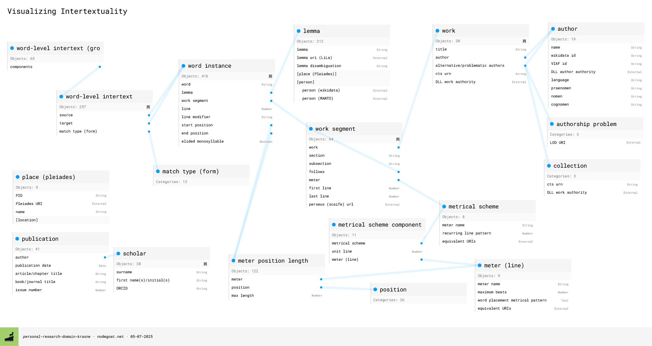
The critical core tables are word instance, word-level intertext, word-level intertext (grouping), author, work, work segment, meter (line), metrical scheme, and meter position length. Each word instance object represents a single word in a single line of a single poem; each word-level intertext object comprises a source word and a target word. Since intertexts are often made up of several words, a word-level intertext (grouping) object clusters these intertext pairings together, taking advantage of nodegoat’s “multiple” option. Words are not assigned directly to works, but to work segments. The way the work segment is determined is due not just to conventional poetic divisions (such as books) but also to meter, because the basis of the intertextual density display is a grid whose width is determined by the meter of the piece. As many works are polymetric, the meter is assigned to the work segment, which can represent anything from an entire work (in the case of, e.g., an epyllion) to a single poem within a multi-book work (e.g., one of Statius’s Silvae) or a passage of a drama (e.g., a section of a choral passage in a Senecan tragedy). A word instance is placed within a work segment by line number and by location within the line, based not on word order or syllable count but on metrical sedes (placement). (This decision was made both to accommodate textual variation and to enable the placement of words within the grid.) The placement is defined by the word’s beginning and ending meter position length objects, which in turn specify the maximum number of beats that can be assigned to a given metrical position: these ultimately govern the appearance of the word in the grid, but they also offer the future possibility of comparing the metrical placement of intertexts. Because metrical patterns potentially appear in a number of different metrical schemes (e.g., a dactylic hexameter line can be used stichically [i.e., repeated line after line], as well as being used in elegiac couplets and some lyric meters, such as Alcmanic strophe), the table metrical scheme component connects individual meters to the metrical scheme that they are part of in order to avoid repetition. (I am not going into detail here on some decisions regarding the calculation of metrical “length” or the properties of various database objects because I hope to publish some of that information in due course; however, it will ultimately be available in some form.)
While the project overall is strictly concerned with Latin poetry, Greek texts also need to be included within the database due to Latin poetry’s clear intertextual engagement with them. Accordingly, each author has a language property that specifies them as either a Greek or Latin author. While this does not allow for the possibility of bilingual authors, our surviving texts do not really compass this scenario, or do so insufficiently to justify putting the language label with works instead of authors. (The Late Antique poet Claudian is one such counterexample, but he is so late that his works are unlikely to serve as the source of any intertexts in the database; and this is the only situation in which a Greek text can enter the database.) Prose texts are also included in the database, but they, like Greek authors, cannot be selected in the interface.
Finally, each word-level intertext records at least one scholarly source for its data (sometimes the original publication proposing the intertext, sometimes a later publication, and sometimes a commentary), sources that are collectively stored in a publication table. (It is also possible to record an ancient work as the scholarly source, since occasionally the explicit recognition of an intertext goes back to a grammarian of antiquity.) This information is made available when a passage is selected.
In addition to the tables described above, the two tables authorship problem and collection are used to model less straightforward forms of authorship (such as anonymity, uncertain authorship, or preservation in a collection of works), while the three tables textual problem, alternate reading, and word-level intertext modification are newer additions to the database that are used to model variant readings and the changes they imply for proposed intertextual allusions. Some additional information about particulars of the database and project can be found on the Frequently Asked Questions page.
Data Pipeline
Non-coders may wish to skip this part!
Data Extraction and Transformation with Python
Every time the website is deployed (usually by an update on GitHub), a data loader written in Python performs an API call to nodegoat to fetch the current database model. It then extracts the nodegoat IDs for each object type table and does another API call for the individual objects. It assigns the objects, under their object types, to a dictionary, and then transforms them into Pandas dataframes, unpacking the highly nested information of the nodegoat JSON objects.
Click here to see the function that performs the extraction.
# Create table dataframes
def table_to_df(table, cols_dict):
    dictlist = []
    for id in table:
        tdict = {}
        obj_defs = table[id]["object_definitions"]
        tdict["obj_id"] = id
        for key, val in cols_dict.items():
            # key becomes key in tdict
            id_val = list(val.keys())[0]
            if val[id_val] == "refid":
                try:
                    refval = obj_defs[str(id_val)]["object_definition_ref_object_id"]
                    if isinstance(refval, list):
                        for i, newval in enumerate(refval):
                            if isinstance(newval, str) and len(newval.split("_")) == 2:
                                splitval = newval.split("_")
                                refval[i] = {'refid': splitval[0],
                                             'refval': splitval[1]}
                            elif isinstance(newval, int):
                                refval[i] = str(newval)
                    tdict[str(key)] = refval
                except:
                    tdict[str(key)] = None
            elif val[id_val] == "objval":
                try:
                    tdict[str(key)] = obj_defs[str(id_val)]["object_definition_value"]
                except:
                    tdict[str(key)] = None
        dictlist.append(tdict)
    df = pd.DataFrame.from_dict(dictlist).copy()

    # catch any exceptions that didn't store empty value as None
    df = df.astype(object)
    df = df.where(~df.isna(), None)

    # convert numeric IDs to string and remove any trailing decimals
    for col in df:
        if col[-3:] == "_id":
            df[col] = df[col].apply(lambda x: str(x) if x is not None else x)
    def remove_decimal(id_string):
        if isinstance(id_string, str) and id_string[-2:] == ".0":
            return id_string[:-2]
        return id_string
    for col in df:
        if col[-3:] == "_id":
            df[col] = df[col].apply(remove_decimal)

    return df
The data loader then joins the disparate metrical data into a single dataframe and returns it to a single restructured JSON object; it also converts each of the other dataframes to a JSON object, which are collectively stored in an array. These are all saved to files that are automatically committed to GitHub.
The same Python data loader also creates network nodes and edges from the data in order to enable visualization of the intertexts as Sankey diagrams. (I chose these over traditional network graphs since the sequential nature of an intertextual network makes it well-suited to visualizing as a flow-path.) While part of the network creation is done automatically by the D3 Sankey module, the initial preparation of nodes and edges is performed in the data loader; further filtering, when necessary, is done on the fly based on the user’s selections.
Click to view the two custom functions for this stage.
grp_intxts_list = [str(item) for sublist in list(word_lvl_intxt_grp_df.word_intxt_ids) for item in sublist]
intxt_grp_list = []

def build_intxt_dict(intxt_ids):
    for intxt in intxt_ids:
        intxt_id = str(intxt)
        for row2 in word_lvl_intxt_df[word_lvl_intxt_df.obj_id == intxt_id].iterrows():
            row_dict = {}
            if intxt_id in grp_intxts_list:
                row_dict["intxt_grp_id"] = intxt_grp_id
            else:
                row_dict["intxt_grp_id"] = None
            row_dict["intxt_id"] = intxt_id
            row2 = row2[1]
            source_id = row2.source_word_id
            target_id = row2.target_word_id
            if isinstance(row2.match_type_ids, list):
                match_type_ids = [str(id) for id in row2.match_type_ids]
            else:
                match_type_ids = []
            row_dict["source_word_id"] = source_id
            row_dict["target_word_id"] = target_id
            source_df = word_instance_df.copy().query(f"obj_id == '{source_id}'").reset_index(drop=True) \
                .merge(work_seg_df, how="left", left_on="work_segment_id", right_on="obj_id").drop("obj_id_y", axis=1) \
                .merge(work_df, how="left", left_on="work_id", right_on="obj_id")[['obj_id_x','word','work_segment_id', 'line_num','line_num_modifier',"work_id","author_id"]]
            target_df = word_instance_df.copy().query(f"obj_id == '{target_id}'").reset_index(drop=True) \
                .merge(work_seg_df, how="left", left_on="work_segment_id", right_on="obj_id").drop("obj_id_y", axis=1) \
                .merge(work_df, how="left", left_on="work_id", right_on="obj_id")[['obj_id_x','word','work_segment_id', 'line_num','line_num_modifier',"work_id","author_id"]]
            row_dict["source_author_id"] = source_df.loc[0,'author_id']
            row_dict["source_work_id"] = source_df.loc[0,'work_id']
            row_dict["source_work_seg_id"] = source_df.loc[0,'work_segment_id']
            if isinstance(source_df.loc[0,'line_num_modifier'], str):
                row_dict["source_line_num"] = str(source_df.loc[0,'line_num'])+source_df.loc[0,'line_num_modifier']
            else:
                row_dict["source_line_num"] = str(source_df.loc[0,'line_num'])
            row_dict["target_author_id"] = target_df.loc[0,'author_id']
            row_dict["target_work_id"] = target_df.loc[0,'work_id']
            row_dict["target_work_seg_id"] = target_df.loc[0,'work_segment_id']
            if isinstance(target_df.loc[0,'line_num_modifier'],str):
                row_dict["target_line_num"] = str(target_df.loc[0,'line_num'])+target_df.loc[0,'line_num_modifier']
            else:
                row_dict["target_line_num"] = str(target_df.loc[0,'line_num'])
            row_dict["match_type_ids"] = match_type_ids
            intxt_grp_list.append(row_dict)

for row in word_lvl_intxt_grp_df.iterrows():
    row = row[1]
    intxt_grp_id = row.obj_id
    intxt_ids = row.word_intxt_ids
    build_intxt_dict(intxt_ids)
build_intxt_dict([intxt for intxt in word_lvl_intxt_df.obj_id if intxt not in grp_intxts_list])

intxt_full_df = pd.DataFrame.from_dict(intxt_grp_list)

def prep_sankey(df):
    nodes_edges_dict = {}
    grp_df = df[~df.intxt_grp_id.isna()]
    no_grp_df = df[df.intxt_grp_id.isna()].drop("intxt_grp_id", axis=1)
    grp_ids = list(grp_df.intxt_grp_id.unique())
    no_grp_ids = list(no_grp_df.intxt_id.unique())
    nodes = []
    edges = []
    for work_seg in list(df.source_work_seg_id.unique()):
        author = df[df.source_work_seg_id == work_seg].reset_index(drop=True).loc[0,"source_author_id"]
        work = df[df.source_work_seg_id == work_seg].reset_index(drop=True).loc[0,"source_work_id"]
        nodes.append({"name": work_seg, "author": author, "work": work})
    for work_seg in list(df.target_work_seg_id.unique()):
        if work_seg not in [item["name"] for item in nodes]:
            author = df[df.target_work_seg_id == work_seg].reset_index(drop=True).loc[0,"target_author_id"]
            work = df[df.target_work_seg_id == work_seg].reset_index(drop=True).loc[0,"target_work_id"]
            nodes.append({"name": work_seg, "author": author, "work": work})
    nodes_edges_dict["nodes"] = nodes
    def make_edge(id, df, grp=True):
        source = df.loc[0, "source_work_seg_id"]
        target = df.loc[0, "target_work_seg_id"]
        source_words = list(df.source_word_id.unique())
        target_words = list(df.target_word_id.unique())
        num_words = (len(source_words)+len(target_words))/2    # using average because sometimes multiple words are compressed into a single word or a single word is split into multiple words
        id = id
        if grp == True:
            group_id = True
        else:
            group_id = False
        edge_dict = {"source": source,
                     "target": target,
                     "source_words": source_words,
                     "target_words": target_words,
                     "num_words": num_words,
                     "id": id,
                     "group_id": group_id}
        return edge_dict
    for id in grp_ids:
        sub_df = grp_df.query(f"intxt_grp_id == '{id}'").reset_index(drop=True)
        edges.append(make_edge(id, sub_df))
    for id in no_grp_ids:
        sub_df = no_grp_df.query(f"intxt_id == '{id}'").reset_index(drop=True)
        edges.append(make_edge(id, sub_df, grp=False))
    nodes_edges_dict["edges"] = edges
    return nodes_edges_dict

sankey_data = prep_sankey(intxt_full_df)
Data Loading and Transformation with JavaScript
The remainder of the code is written in JavaScript, within an Observable Framework markdown document. After loading the data, the script defines several inputs for the choice of author, work, work section, and lines. Each is dependent on the selection made in the previous one, so that the data is progressively filtered.
Click to view the code for the Author, Work, and Work Section selectors
N.B. I have removed indications of separate code blocks from the following, although Observable Framework requires each dropdown to be created in a separate block in order to use the information from the previous dropdown.
// Create authors dropdown

const authorList = [];
const authorTable = nodegoatTables.author_table;

// filter to authors that have written poetry in plottable meters
let workSegFilter = nodegoatTables.work_seg_table.filter(workSeg => workSeg.meter_id !== proseID).map(workSeg => workSeg.work_id);
let workFilter = nodegoatTables.work_table.filter(work => workSegFilter.includes(work.obj_id)).map(work => work.author_id);

let authorFilter = nodegoatTables.author_table.filter(author => workFilter.includes(author.obj_id));

for (let author in authorFilter) {
	if (authorFilter[author].language === "Latin") {
		const authorSet = [authorFilter[author].author_name, authorFilter[author].obj_id];
		authorList.push(authorSet);
	}
}

// Add catch-all for works without an assigned author
authorList.push(["Anonymous works", "000"]);

authorList.sort((a,b) => d3.ascending(a[0], b[0]));

const authorPicker = Inputs.select(new Map([[null,null]].concat(authorList)), {label: "Select author:", value: null, sort: false});
const authorID = view(authorPicker);


// Create works dropdown

const workList = [];
const workTable = nodegoatTables.work_table;

for (let work in workTable) {

	if ((workTable[work].author_id === authorID && workTable[work].author_id) || (authorID === "000" && !workTable[work].author_id)) {
		const workSet = [workTable[work].title, workTable[work].obj_id]
		workList.push(workSet);
	}

	// if an anonymous work is traditionally (but probably incorrectly) attributed to an author, also add it to their list of works, but with the title in brackets
	else if (workTable[work].authorship_prob_ids) {
		let altAuthorPossibilities = workTable[work].authorship_prob_ids.filter(problem => problem.refid === "21843").map(alt => alt.refval);

		if (altAuthorPossibilities.includes(authorID)) {
			const workSet = [`[${workTable[work].title}]`, workTable[work].obj_id]
			workList.push(workSet);
		}
	}

}

workList.sort((a,b) => d3.ascending(a[0], b[0]));

const workPicker = Inputs.select(new Map([[null, null]].concat(workList)), {label: "Select work:", value: null, sort: false});
const workID = view(workPicker);


// Create work section dropdown

const workSegList = [];
const workSegTable = nodegoatTables.work_seg_table;

for (let workSeg in workSegTable) {
	let workSegName;
	if (!workSegTable[workSeg].work_section) {
		workSegName = "all"
	} else if (!workSegTable[workSeg].work_subsection) {
		workSegName = workSegTable[workSeg].work_section;
	} else {
		workSegName = workSegTable[workSeg].work_section + ', ' + workSegTable[workSeg].work_subsection;
	}

	if (workSegTable[workSeg].work_id === workID) {
		const workSegSet = [workSegName, workSegTable[workSeg].obj_id];
		workSegList.push(workSegSet)
	}
}

workSegList.sort((a,b) => a[0].localeCompare(b[0], undefined, {numeric: true}));

const workSegPicker = Inputs.select(new Map([[null, null]].concat(workSegList)), {label: "Select work section:", value: null, sort: false});
const workSegID = view(workSegPicker);
The creation of the two inputs for choosing the starting and ending lines for display required slightly more complex logic, as it needed to be based both on what was available to display in the chosen work section while also providing some default inputs.
Click to view the code for choosing the starting and ending lines
N.B. I have removed indications of separate code blocks from the following.
// Create necessary variables for chart display

const workSegVars = {
	workSegLineMin: 1,
	workSegLineMax: null,
	workSegMeterID: null
};

// Set variables for chart display, based on work segment chosen

for (let workSeg in workSegTable) {
	if (workSegTable[workSeg].obj_id === workSegID) {
		workSegVars.workSegLineMin = workSegTable[workSeg].first_line;
		workSegVars.workSegLineMax = workSegTable[workSeg].last_line;
		workSegVars.workSegMeterID = workSegTable[workSeg].meter_id;
		break;
	}
}

// Create number pickers for range of lines to display

const lineMinPicker = Inputs.number([workSegVars.workSegLineMin, workSegVars.workSegLineMax],
									{step: 1,
									label: "Select starting line: ",
									value: workSegVars.workSegLineMin,
									placeholder: workSegVars.workSegLineMin});
const startLine = view(lineMinPicker);

let tempMax = Math.min(workSegVars.workSegLineMin + 19, Math.max(workSegVars.workSegLineMin,workSegVars.workSegLineMax))

const lineMaxPicker = Inputs.number([workSegVars.workSegLineMin, workSegVars.workSegLineMax],
									{step: 1,
									label: "Select ending line: ",
									value: tempMax,
									placeholder: workSegVars.workSegLineMax});
const endLine = view(lineMaxPicker);

// Set default numbers

const lineRange = {
	firstLine: 1,
	lastLine: function() {return this.firstLine + 20;},
}


if (startLine > 0) {
	lineRange.firstLine = startLine;
}

if (endLine >= startLine) {
	lineRange.lastLine = endLine;
} else {lineRange.lastLine = lineRange.firstLine + 0;}
Once the passage is chosen, the script gathers any word instance that falls within the selected lines and then filters the word level intertext objects for those that include the relevant words as an intertext target. These are considered “direct intertexts”. It then collects any intertexts where the source of a direct intertext is the target, and so on; all of these are considered “indirect intertexts”. An empty grid is generated with Plot.cell, using the number of selected lines for its height and the relevant meter’s maximum length for its width. Each cell of the grid is populated with the relevant word and intertext counts for that line and metrical position.
Click to view the code for building the grid.
// Define grid width based on the selection's meter.

let gridX;

for (let meter in meters) {
	if (meters[meter].metrical_scheme_id === meterID) {
		gridX = meters[meter].max_line_beats;
	}
}

// Define grid height based on number of lines.

let gridYInterim = (lineRange.lastLine - lineRange.firstLine) + 1;
let extraLineSet;

// make a set of any extranumerical lines

if (wordsFiltered.filter(word => word.line_num_modifier).length > 0) {
	extraLineSet = new Set(
		wordsFiltered.filter(word => word.line_num_modifier)
					.map(word => ({lineNum: word.line_num, lineNumMod: word.line_num_modifier, lineNumString: `${word.line_num}${word.line_num_modifier}`}))
	);
	gridYInterim += extraLineSet.size;	// if there are extranumerical lines, increase the height multiplier accordingly, so that cells remain square
}

const extraLines = extraLineSet ? Array.from(extraLineSet) : [];

const gridY = gridYInterim;

const cellSize = 20;
const gridHeight = gridY * cellSize;
const gridWidth = gridX * cellSize;


// Create plot, conditional on the existence of intertexts

// set tick range; increase step every ten (max) intertexts
let step;
if (d3.max(intxtCnts)%10 === 0) {
	step = d3.max(intxtCnts)/10;
}
else {
	step = Math.floor(d3.max(intxtCnts)/10) + 1;
};
let tickRange = d3.range(Math.min(...intxtCnts), Math.max(...intxtCnts)+1, step);

let lineVals = d3.range(lineRange.firstLine, lineRange.lastLine +1);

// if there are extranumerical lines, insert them into the line values array

for (let line of extraLines) {
	let insertAfter = line.lineNum;
	let insertAfterIndex = lineVals.indexOf(insertAfter) + 1;
	let insertString = line.lineNumString;
	lineVals.splice(insertAfterIndex, 0, insertString);
}


const plotDisplay = intertextsArr.every(intxt => intxt.intxtCnt === 0) ? null : Plot.plot({
	grid: true,
	x: {
		label: null,
		domain: d3.range(1,gridX+1),
		padding: 0,
		axis: null,
		},
	y: {
		label: 'Line',
		// domain: d3.range(lineRange.firstLine, lineRange.lastLine +1),
		domain: lineVals,
		tickSize: 0,
		},
	color: {scheme: "Greens",
		legend: true,
		label: "Total Intertexts (direct & indirect)",
		ticks: tickRange,
		tickFormat: d => Math.floor(d),
		},
	marks: [
		Plot.cell(intertextsArr, {
			x: "linePos",
			y: "lineNum",
			fill: d => d.wordObj.directIntertexts + d.wordObj.indirectIntertexts,
			tip: {format: {
				word: true,
				x: false,
				y: false,
				lineNum: true,
				fill: false
			}},
			channels: {
				title: d => `${d.wordObj.word} (line ${d.lineNum})\n# direct intertexts: ${d.wordObj.directIntertexts}\n# indirect intertexts: ${d.wordObj.indirectIntertexts}`,
				word: d => d.wordObj.word,
				lineNum: {
					value: "lineNum",
					label: "line"
				},
				dirIntxt: {
					value: d => d.wordObj.directIntertexts,
					label: "# direct intertexts"
				},
				indIntxt: {
					value: d => d.wordObj.indirectIntertexts,
					label: "# inherited intertexts"
				},
			},
		})
	],
	style: {fontSize: "12pt"},
	width: gridWidth + 120,
	height: gridHeight + 50,
	marginTop: 20,
	marginRight: 50,
	marginBottom: 30,
	marginLeft: 70
});
The Sankey diagrams, in turn, are generated by a function that is (increasingly heavily) modified from the D3 library’s Sankey module. The main modifications, other than rotating the diagram to flow top-to-bottom, lie in the mouseover interactions (highlighting and informational tooltip popups). However, while the input data for the full intertext diagram already exists (generated by the data loader, as discussed above), and the input data for the passage-level diagram (described below) is for the most part just a filtered version of the fuller data, the input data for the Sankey chart that is generated when a word is clicked on (also described below) needs to be built on the fly.
Click to view the code for building the word-level Sankey chart nodes and links.
// data prep for chart if a word is selected: Sankey based on word-to-word connections

const ancestorIntertexts = [];
const descendantIntertexts = [];

let currWordId;
let ancestorWordIDs = [];
let descendantWordIDs = [];

if (plotCurrSelect) {

	currWordId = plotCurrSelect.wordObj.obj_id;	// set current word ID to the selected word

	let intertextsTableExtended = intertextsTable.concat(intertextsModTable);

	// create functions for getting a word's immediate ancestors or descendants
	function getWordAncestors(currWordId){
		for (let i in intertextsTableExtended) {
			let intxt = intertextsTableExtended[i];
			// for each intertext in the intertexts table, if its target ID matches the focus word (either the selected word or one of its ancestors), add it to the list of ancestor intertexts and add its source to the list of words to be processed.
			if (currWordId === intxt.target_word_id) {
				ancestorIntertexts.push(intxt);
				ancestorWordIDs.push(intxt.source_word_id);
				wordSankeyIntxtIDs.push(intxt.intxt_id);
			}
		}
	}
	function getWordDescendants(currWordId){
		for (let i in intertextsTableExtended) {
			let intxt = intertextsTableExtended[i];
			// for each intertext in the intertexts table, if its source ID matches the focus word (either the selected word or one of its descendants), add it to the list of descendant intertexts and add its target to the list of words to be processed.
			if (currWordId === intxt.source_word_id) {
				descendantIntertexts.push(intxt);
				descendantWordIDs.push(intxt.target_word_id);
				wordSankeyIntxtIDs.push(intxt.intxt_id);
			}
		}
	}

	getWordAncestors(currWordId);
	getWordDescendants(currWordId);

	while (ancestorWordIDs.length > 0) {
		currWordId = ancestorWordIDs[0];
		getWordAncestors(currWordId);
		ancestorWordIDs.shift();
	}

	while (descendantWordIDs.length > 0) {
		currWordId = descendantWordIDs[0];
		getWordDescendants(currWordId);
		descendantWordIDs.shift();
	}
}

const intertextsWordFiltered = Array.from(new Set(ancestorIntertexts.concat(descendantIntertexts)));

const wordIntxtNodeIDs = Array.from(new Set(intertextsWordFiltered.map(intxt => (Object.values({source_word_id: intxt.source_word_id, target_word_id: intxt.target_word_id}))).flat()));

let wordInstanceTable = JSON.parse(JSON.stringify(nodegoatTables.word_instance_table));
const wordIntxtNodes = wordIntxtNodeIDs.map(id => wordInstanceTable.filter(word => word.obj_id === id)[0]);
wordIntxtNodes.forEach(obj => obj.id = obj.obj_id);
wordIntxtNodes.forEach(obj => delete obj.obj_id);
for (let i in wordIntxtNodes) {
	if (wordIntxtNodes[i].id === plotCurrSelect.wordObj.obj_id) {
		wordIntxtNodes[i].color = "#0088ff";
	}
}

const wordIntxtEdges = [];

for (let i in intertextsWordFiltered) {
	let intxt = intertextsWordFiltered[i];
	wordIntxtEdges.push({source: intxt.source_word_id, target: intxt.target_word_id, value: 1, id: intxt.intxt_id, matchTypes: intxt.match_type_ids});
}
Visualizations
The main visualization is intended to resemble the layout of the poem, for purposes of familiarity and visual analysis. It shows the density of intertexts that stand behind each word of the poem. While the accuracy of the display is naturally conditional on the contents of the database, it will ultimately allow users to ask questions such as “where in these lines are intertexts concentrated?” Instructions for reading the chart — including reminders of the data’s incompleteness — are presented alongside.
Also displayed on the main page are two Sankey diagrams — one shown by default, as soon as a passage is selected, and one shown once the user selects a word in the main “poem” visualization. These both show the intertextual “family tree,” one showing the texts that stand behind the selected passage, and the other showing the individual words in other poems that have intertextual connections with a single, selected word. The first of these is a filtered version of the diagram that can be viewed on the Full Intertext Diagram page. All the Sankey diagrams have popups to provide the user with additional information.
The colors that are used to distinguish between authors in the passage-level and full intertext diagrams are drawn from the Glasbey colormap provided by the Python library colorcet. While the Glasbey colors are perceptually dissimilar to the extent possible, a large number of authors will still cause difficulty in distinguishing between shades; accordingly, they are reinforced by the inclusion of the author’s name. (The names are rotated sideways in order not to overrun the boundaries of smaller nodes; this study on the readability of tilted text suggests that there is not a significant difference in the readibility of sideways text read top-to-bottom or bottom-to-top.)
Next Steps
The main focus for the near future is on entering additional intertexts into the database. Once sufficient intertexts have been entered, work can begin on the creation of analytical tools, enabling researchers to ask and answer questions about the data.
A few additional, potential, long-term developments are:
- an option to view only direct intertext density
- an option to view “descendant” intertexts instead of “ancestor” intertexts in the density display
- collaboration with projects on automated detection of text reuse (such as Tesserae or Fīlum) to enhance the database, with a reduction of manual labor
Other requests and suggestions for future development are welcome at the GitHub page.
Bibliography
- Dexter, J.P., Chaudhuri, P., Burns, P.J., Adams, E.D., Bolt, T.J., Cásarez, A., Flynt, J.H., Li, K., Patterson, J.F., Schwartz, A., Shumway, S. (2024) “A Database of Intertexts in Valerius Flaccus’ Argonautica 1: A Benchmarking Resource for the Evaluation of Computational Intertextual Search of Latin Corpora,” Journal of Open Humanities Data 10:14, 1–7. doi: 10.5334/johd.153
- Hardie, P. R. (1989) “Flavian Epicists on Virgil’s Epic Technique,” Ramus 18: 3–20.
- Thomas, R.F. (1986) “Virgil’s Georgics and the Art of Reference,” Harvard Studies in Classical Philology 90: 171–98.
Appendix: Getting Started with Observable Framework
In learning how to use Framework and setting up my site, I encountered a few snags with the default installation setup and automated deployment via GitHub, which I document here for others who may encounter the same issues.
- First, while following the Learn Observable Guide, I kept running into an error that claimed I didn't have Python installed when I tried to use a data loader that I had written in Python. The problem turned out to be that my computer runs Python with
pythonrather thanpython3, and the latter is the only possibility recognized by theobservablehq.config.jsfile. The solution is to add the following to the end of the file, just before the closing};:
// MODIFY LIST OF INTERPRETERS:
  interpreters: {
	".py": ["python"]
  },
- Second, after setting up an automated deployment using GitHub Actions every time I pushed changes to GitHub, I encountered two problems. First, because I was importing a couple of packages in my Python data loader, I was getting an error message when running the build that the package wasn't found, a problem that had already been documented and solved here. But even after following the documented steps, I continued to get the error message, and GitHub was telling me that the deploy had failed, but without an actual failure (i.e., the site was correctly updating on Observable Framework). The solution was to also add a new line to Framework's
package.jsonfile:
// ...
"observable": "observable",
"install": "pip install -r requirements.txt"    // this is the new line
// ...
- Third, when using GitHub Actions and a
deploy.ymlscript for an automated deploy, any API keys need to be added to both Observable Framework secrets and GitHub Secrets, as well as adding them in the build step of thedeploy.ymlscript:
- run: npm run build
  env:
    NODEGOAT_API_TOKEN: ${{ secrets.NODEGOAT_API_TOKEN }}
- Fourth, I needed my data loader to produce multiple files, not just the one it’s intended to produce at the end, due to needing to limit my API calls (I have enough tables to retrieve from nodegoat that I can only call the full set of them once every fifteen minutes). This was in itself not a problem, but the files weren't storing themselves successfully on GitHub. I ultimately discovered (with the aid of ChatGPT to get the exact correct format) that I needed to add yet another step to my
deploy.ymlscript; and I also needed to add a GitHub token to both the build step and the new commit/push step, so that this portion of the script looked as follows:
- run: npm run build
  env:
    NODEGOAT_API_TOKEN: ${{ secrets.NODEGOAT_API_TOKEN }}
    GITHUB_TOKEN: ${{ secrets.GITHUB_TOKEN }}
- name: Commit and Push Changes
  run: |
    git config --global user.name "GitHub Actions"
    git config --global user.email "actions@github.com"
    git add .
    git diff --quiet && git diff --staged --quiet || git commit -m "Auto-update model_json_backup.json and objects_json_backup.json"
    git push
  env:
    GITHUB_TOKEN: ${{ secrets.GITHUB_TOKEN }}
An alternative approach to this might have been to output a .zip file instead of a JSON file from the data loader, since Observable Framework can attach files directly from a zip archive.